Welcome to the Frequently Asked Questions (FAQ) page. This page is designed to
be your first approach in finding answers to common questions on mixing zones
and how CORMIX models them.
So there is no need to "flame-out" like the guy on the right-
just keep cool and check out the links below.
Please don't hesitate - send us your ideas on how we might make this FAQ more responsive to your needs.

CORMIX Frequently Asked Questions (FAQ) |
|||
|
|
%20copy.jpg)
A fire-breather demonstrates the principles of Buoyant Jet Mixing
|
||
|
A.
CORMIX software is licensed and distributed solely by MixZon Inc The first step to licensing CORMIX on your computer is to install the free evaluation version. The latest software release contains new tools for mixing zone analysis, updated hydrodynamics, and mixing zone decision support.
The downloads page contains links to the free evaluation
version CORMIX v12.0E. The evaluation version can then be activated/unlocked to commercial
versions after buying appropriate license/s from MixZon Inc.
**PLEASE NOTE**
A. The complete CORMIX User Manual (in Adobe Acrobat - PDF format) is available for download, using your MixZon account information from the downloads site (approximately 25.0 Mb).
The User Manual is also part of the CORMIX installation. If you have installed CORMIX v12.0 on your system, the User Manual is located in the installation directory under the ..\docs sub-directory as the file "User_Manual.pdf".
A. Check the technical support page for additional details. The general procedure is as follows. If you are using CORMIX you will need to locate the corresponding input data file(s) (fileid.cmx) for each case under consideration. You should send this file(s) as an email attachment (no need to compress or alter) with specific questions regarding each case to the contact listed below. When making inquiries, please refer to specific cases and flow module regions within your prediction file(s) (fileid.prd). Please send help requests within email text or as Adobe Acrobat attachments. Attachments such as Word documents are not accepted because of security risks in opening these files. Legacy DOS/Windows versions of CORMIX and versions less than the current version, CORMIX v12.0, are NOT supported. A. CORMIX applications include the most common wastewater discharges where initial mixing zone characteristics are desired. The User Manual has a good primer on initial mixing processes in general and how CORMIX models them in particular. Also, the links on this website should be helpful. In particular, near-field, boundary interaction, and far-field mixing processes should be thoroughly explored. Pay attention to stable versus unstable flow processes, near-field dynamic attachments, and the schematization of data for CORMIX data entry. The sections on applications and the image gallery should also be examined. Furthermore, look at CORMIX1, CORMIX2, and CORMIX3 system descriptions.
In addition, you can download the evaluation version of CORMIX and determine if CORMIX
applies to your case. The evaluation version software allows a no-risk evaluation/demonstration of program capabilities. A. Most successful CORMIX model users have a background in physical sciences and/or engineering. Many people apply the model successfully after carefully reading the User Manual and closely following the case studies presented in Appendices B, C, D, and E. Also, the links on this website may be useful. Please check the training page for scheduled CORMIX workshops. Please refer to the CORMIX installation Troubleshooting Guide, for help related to this issue. The save and print features have been DISABLED in the evaluation/demo version of CORMIX. You will need a valid, licensed version of CORMIX to save and print CORMIX output under Windows reliably.
You can save and print the output from the visualization tools like CorVue and CorSpy, directly, from within their respective UIs, using the Save As and Print toolbar buttons. A. Yes, updated hydrodynamic models are used in all software release versions. Specifically, CORMIX1 and CORMIX2 simulation algorithms were modified for terminal level behavior in density stratified crossflow and for representation of the following asymptotic flow regimes: pure jet, pure plume, pure wake, and advected line puff. Additional details about the asymptotic flow regimes can be found in a paper by Jirka, 1999. The CORMIX3 simulation models were extensively revised replacing many near-field analytic solutions with an integral model approach. Also, CORMIX predictions are within +/- 50% of one standard deviation of available data. When comparing predictions, dilution S should be used for comparison, not concentration. Furthermore, when comparing dilution S values, use the Logarithm of dilution S. All Log10(S) are well within the scatter of associated field and laboratory data. The CORMIX software is continuously updated with new and improved features, updated hydrodynamics, rule-bases, and fixes for reported bugs. These are documented as part of the CORMIX Quality Assurance - New Features, Updates & Fixed Bug List, published on the MixZon website at http://www.mixzon.com/quality_assurance.php.
Q.9. How do I interpret plume dimension values and how can I compute/plot plume concentration isoline profiles?
A. The CORMIX User Manual shows plume width and profile definitions in Figure 5.5, and additional advice on plotting isoline concentrations appears on page 76 (New User Manual - 2007 v5.4). The FORTRAN prediction files (e.g. fileid.prd) list the plume profile definitions used within each module at the beginning of the output for each module. Plume horizontal width values (BH) are reported as half-widths until bank contact, after which they are reported as full widths. After bank contact, the plume centerline coordinates switch to the contacted bank, which then becomes a plane of symmetry. Also, in most mixing zone analysis, minimum centerline dilution is often the only acceptable parameter to determine regulatory compliance. The CorVue visualization tool available in CORMIX gives 3-D and 2-D visualizations of minimum centerline concentration, flow dimensions, and regulatory mixing zone compliance.
Q.10. How do I account for an ambient background concentration of a pollutant in the receiving water?
A. As a mixing zone model, CORMIX assumes that sufficient ambient water is available to dilute the effluent to levels that approach the background concentration. Thus it is assumed that the volume flux (m3/s) of the discharge Q0 is much less than the volume flux of the ambient Qa (i.e. Q0 << Qa). If the above volume and mass flux assumptions hold, then advice for simulating cases with ambient background concentrations as excess concentrations appears in the CORMIX User Manual as an example on page 61 (New User Manual - 2007 v5.4). A. CORMIX does not have any user-adjustable parameters. However, it is suggested that you run a sensitivity analysis representing a range of discharge (velocity, density) and/or environmental conditions (depth, velocity, density stratification) likely to occur at your site. The advanced post-processing tool CorSens available in CORMIX v12.0GT can automatically create input files and execute batch simulations for sensitivity study analysis and outfall design. This tool allows the analyst to quickly assess boundary interaction and stability as well as regulatory mixing zone properties including CCC compliance for a range of discharge and ambient conditions. A. In cases with steady ambient flows, check the prediction file (fileid.prd) for warning messages about limiting dilutions and/or low ambient velocities. If the ambient velocity is very small (or zero), unsteady ambient flow processes may cause pollutant build-up in the near-field. Therefore the flow behavior and thus dilution will be highly dependent on local ambient geometry. There are no general modeling approaches to determine far-field mixing zones in these low ambient velocity cases. However detailed numerical models may be applied, but the time and expense involved often make these numerical modeling approaches impractical. In cases with unsteady ambient environments, CORMIX is a steady-state model, whereas tidal cycles are an inherently unsteady ambient environment. In tidal mode, CORMIX accounts for the re-entrainment of the historic plume remaining from the previous tidal cycle. Because it takes time for the historic plume to develop, there is a limited region/time over which this re-entrainment will occur.
Q.13. How does CORMIX simulate tidal re-entrainment?
A. CORMIX is a steady-state model, whereas tidal environments are inherently unsteady. Because most regulatory mixing zone analysis requires "worst-case" dilution analysis, analysts sometimes consider conditions at slack tide (often zero ambient velocity) as representative of the "worst-case". However, minimum initial dilution generally will not occur at slack tide, but shortly after slack tide when the plume re-entrains material remaining from the previous tidal cycle. In tidal mode, CORMIX considers the reduction in initial dilution due to the re-entrainment of material remaining from the previous cycle. It does not consider unsteady build-up of material over several tidal cycles, it assumes complete flushing of the historic plume in the near-field, will occur within a tidal cycle. If unsteady build-up in the near-field or far-field over multiple tidal cycles is likely at your site, additional methods of analysis may be necessary. Section 8.6 in Technical Guidance Manual for Performing Waste Load Allocations Book III: Estuaries Part 3 Use of Mixing Zone Models in Estuarine Waste Load Allocations (EPA 823-R92-004) discusses the calculation of pollutant build-up over multiple tidal cycles. A. If you are using CORMIX v12.0, a popup window will appear stating that you should e-mail your input file to support@mixzon.com. If you get a message that says "traceback error", "what is the FLOAT value for GPO . .", or "what is the value of . . .". In such cases, please send the corresponding data input file (fileid.cmx) as an attached file to technical support with a note about the case. A vast majority of simulations will execute within seconds, however, depending on the flow classification and your computer configuration, some simulations may take up several hours.
For the "INPDATA" error - please refer to our FAQ at:
A. The CORMIX1 and CORMIX2 Technical Reports are currently available in
hard copy format only through NTIS.
However, a complete CORMIX documentation set is available from MixZon Inc in online hypertext format. This product - CorDocs- is available in CORMIX v12.0G/GT/GTH/GTS/GTD/GTR and contains the CORMIX1 and CORMIX2 USEPA technical reports as well as the CORMIX3 technical report from the DeFrees Hydraulics lab. Please, check the CORMIX downloads page for additional information. A. In CORMIX, wind velocity specification is used for two purposes:
Therefore, in general, wind is not a directional quantity within CORMIX but is used to adjust density current mixing properties. The required CORMIX ambient schematization assumes a surface velocity field in only one direction. If winds affect the ambient velocity field direction, that information should be captured by your schematization, where the wind-induced ambient velocity direction is specified as the positive x-axis direction. However, if you have a directionally non-uniform ambient velocity profile and a stable CORMIX flow classification, then CorJet may be applied for detailed near-field turbulent buoyant jet mixing in such a directionally non-uniform velocity field. This application is specified by using skewed velocity profiles. See Appendix E of the CORMIX User Manual for an example application of near-field mixing analysis with a directionally skewed ambient velocity profile. A. No. This simply reflects a misunderstanding about the mechanisms controlling multiport diffuser mixing. Mixing in multiport diffusers after plume merging is primarily controlled by the flux of momentum and buoyancy per unit of diffuser length in relation to the local layer depth Hs. Thus, CORMIX uses the primary controlling variable of flux per length of the diffuser, not the number of ports to determine mixing behavior. Changing the number of ports will not affect CORMIX flow classification or dilution estimates of near-field mixing after plume merging occurs. However, changing the diffuser length can sometimes have a strong influence on mixing behavior. For instance, in density-stratified ambients, changing the diffuser length can affect flow trapping behavior and density current terminal level formation. CORMIX will alert the analyst to a flow class change when altering diffuser length. A. No, most certainly not. CORMIX is just reflecting the fact that mixing processes do not always behave in a continuous manner. These phenomena are well supported by experimental data, and CORMIX simply reflects their occurrence. Flow processes can be unsteady because mixing is a turbulent and often chaotic process, where small changes in initial conditions can affect mixing behavior. Since CORMIX (like all other models) assumes steady-state discharge conditions, some jumps in dilution prediction may occur when changing ambient or discharge variables that force a transition from one flow class to another flow class. Therefore, some jumps in dilution may occur in sensitivity analysis when a change in discharge or ambient conditions causes a change in flow classification, i.e. a flow class transition. In reality, such a flow class transition in nature will tend to be an unsteady process. In such an unsteady transition, the observed flow process (e.g. a density current upstream intrusion) may appear, dissipate, and then reappear again over time in an unsteady manner. However, within a given flow class simulation, CORMIX will always give continuous dilution predictions between flow module regions. However, sometimes flow width predictions will experience a jump between flow module regions. This is largely an artifact based upon the definition of the plume width (i.e. concentration profiles based upon maximum centerline versus flux averaged). The concentration profile definition is largely an arbitrary quantity selected for mathematical convenience rather than for the significance of some underlying physical effect. The most important points are that i) changes in mixing behavior are supported by available data, and ii) CORMIX alerts the analyst to the change in mixing behavior with its extensive program documentation. Thus, the savvy analyst will view this as evidence of the robust nature of CORMIX and should consider it carefully in diffuser design. Other available models would not even indicate the possibility of a change in physical mixing behavior when changing discharge or ambient variables (e.g. when changing diffuser length or discharge density), and therefore may give "comforting" but misleading continuous dilution predictions. A. There are a host of distinct differences in usability, range of application, physical processes simulation, and modeling philosophy. A few of them are listed below.
In summation, situations where both CORMIX and PLUMES can be applied would typically be deep ocean outfalls where near-field mixing is of interest only, and there is no possibility of dynamic bottom attachments. However, there is no procedure within PLUMES to test for the possibility of bottom-attached flows. In addition, if mixing zone information after the near-field is desired, then the possibility of a density current in the far-field must be considered. Again, there is no procedure within PLUMES to model density current mixing. Only CORMIX contains rule-based documentation of procedures to test for bottom attached flows and density current mixing. A. YES, CORMIX can be used to model river mixing of oil emulsions. However, CORMIX does not simulate the mixing of multiphasic liquids consisting of two or more immiscible liquid phases. Please download the free evaluation version of CORMIX, CORMIX v12.0E, from the downloads page at MixZon Inc to determine if CORMIX applies to your case/study.
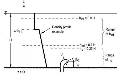
A. YES, CORMIX can be used to model "submerged but elevated discharges" where the port is NOT Deeply Submerged (H0 <= 1/3HD) nor is it Near Surface (H0 >= 2/3HD), i.e.
the port elevation (H0) is such that 1/3HD < H0 < 2/3HD.
The above applicability criterion of port height (H0) and the depth at discharge (HD) in CORMIX is needed to assure a valid test for discharge stability (deep/stable or shallow/unstable flow conditions) in the flow classification scheme. If the discharge is well submerged but 1/3HD < H0 < 2/3HD (i.e. a "submerged but elevated discharge"); CORMIX can still be used in the following iterative fashion by the process of proper analysis and schematization: Case i) For a strongly, positively buoyant jet that tends to quickly rise to the surface, assume that the bottom lies higher so that the port elevation (H0) relative to the "reduced depth" meets the H0 <= 1/3 HD criterion. The CORMIX predictions with this new schematization will be valid if they indicate a stable flow class for this "reduced depth" condition without any unstable recirculation or bottom attachments. If the model predicts an attached flow class, try to re-schematize the bottom, while meeting the above criterion. Case ii) For a strongly negatively buoyant jet that tends to rapidly sink towards the bottom, assume the water surface is "sufficiently higher" so that the port elevation (H0) meets the H0 <= 1/3 HD criterion. Evaluate the CORMIX predictions to check for stable discharge configurations that would not interact with the actual water surface. If the model predicts surface interaction with the schematized water surface, try to re-schematize the water surface, while meeting the above criterion. Case iii) If unstable discharge conditions are expected or predicted (this would be indicated if the above assumptions are violated) then the actual port elevation (H0) is frequently of secondary importance, while water depth (HD) is the primary parameter. In this case, a reduced port elevation meeting the H0 <= 1/3HD limits can be specified for modeling purposes. The experienced user will proceed with careful, iterative evaluation of such complex, and perhaps unusual, "submerged but elevated discharge" cases.
Q.22. The water quality of the effluent is better than that of the river. The discharge concentration input to CORMIX is the concentration above the ambient level.
Is there a way to use CORMIX in this situation?
A. YES, CORMIX can be used in such scenarios.
Q.23. How do I convert CORMIX predicted plume centerline dilutions (Sc) to flux averaged (bulk) dilutions (Sf) and vice versa?
Please use the following conversions to convert between CORMIX predicted flux-averaged and plume centerline dilutions:
Q.24. Why does CORMIX data input validation check that the actual depth at the discharge location (HD) does not differ from the average ambient depth (HA) by more than +/- 30%?
CORMIX is a steady-state, near-field model that assumes a uniform ambient flow field within the schematized ambient cross-section.
Q.25. Why does the CORMIX model require that the input value of multiport diffuser length (LD) be greater than the input local layer depth (HD)?
To have line source mixing behavior (multiport diffuser) in a uniform ambient, the multiport diffuser length LD must be equal to or greater
than the depth HD at discharge. In a stratified ambient, LD must be greater than or equal to the applicable layer depth (HS).
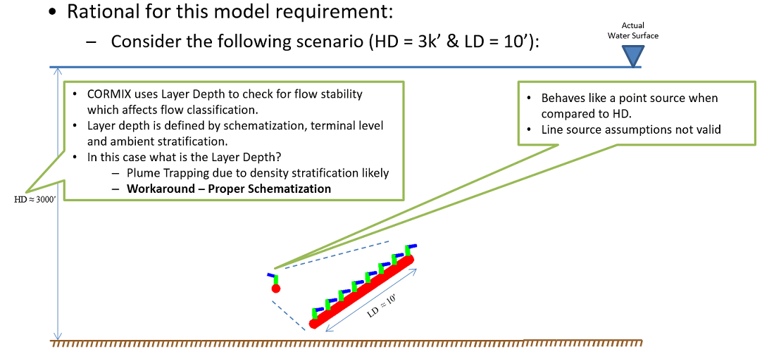
An example to explain the rationale as to why CORMIX requires input LD >= HD (HS)
According to a Wikipedia article: 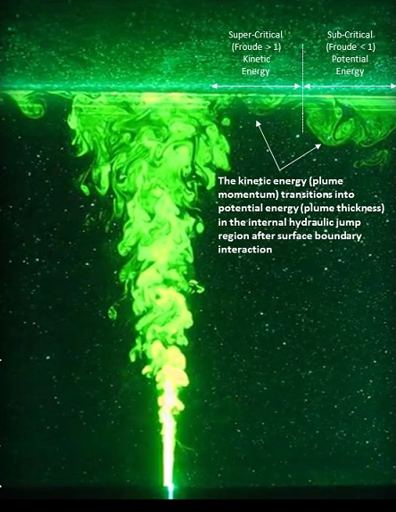
A Vertical Buoyant Jet, 3DLIF actual experiment by Dr. Philip Roberts and Ozeair Abessi, Georgia Institute of Technology.
The image shows internal hydraulics jumps after boundary interaction and during the transition to far-field. In certain CORMIX simulations, the initial predicted plume width values from the end of the near-field are corrected in the next predicted far-field module to conserve the mass flux in the far-field. When the computed correction factor is quite large, it is usually due to the small ambient velocity relative to the strong mixing characteristics of the discharge. In such cases, CORMIX predicts localized RECIRCULATION REGIONS and INTERNAL HYDRAULICS JUMPS and concludes that the predicted flow appears to be highly UN-STEADY in the transition to the far-field and that the predicted far-field transition results MAY be unreliable. The end-user is requested to carefully evaluate the level of near-field lateral boundary interaction when reviewing simulation results.
For Bounded Ambient Cross-Sections, LIMITING DILUTION, SLIM = (QA/Q0) + 1 where
The LIMITING DILUTION is the maximum available physical dilution for the schematized input ambient cross-section.
When the CORMIX model predicts a dilution value that is greater than SLIM, it provides a limiting dilution warning as follows:
The CORMIX model provides you with plume centerline trajectory and physical dilution S = C0/C where,
Q.29. Why does CORMIX require a minimum of 3 ports for multiport diffuser specification and modeling?
CORMIX input data validation requires that the number of ports (NOPEN) is a minimum of 3 when modeling multiport diffuser line sources. While two points in geometry define a “line”, two ports do not typically represent “line source” conditions for mixing zone modeling and outfall design modeling purposes. Diffusers with 3 ports or less are typically not recommended for practical and performance reasons. However, we do recommend diffuser line source assumption verification with CorHyd for all CORMIX mixing zone modeling projects. One should determine line source physical properties to evaluate discharge stability and near-field plume merging behavior. 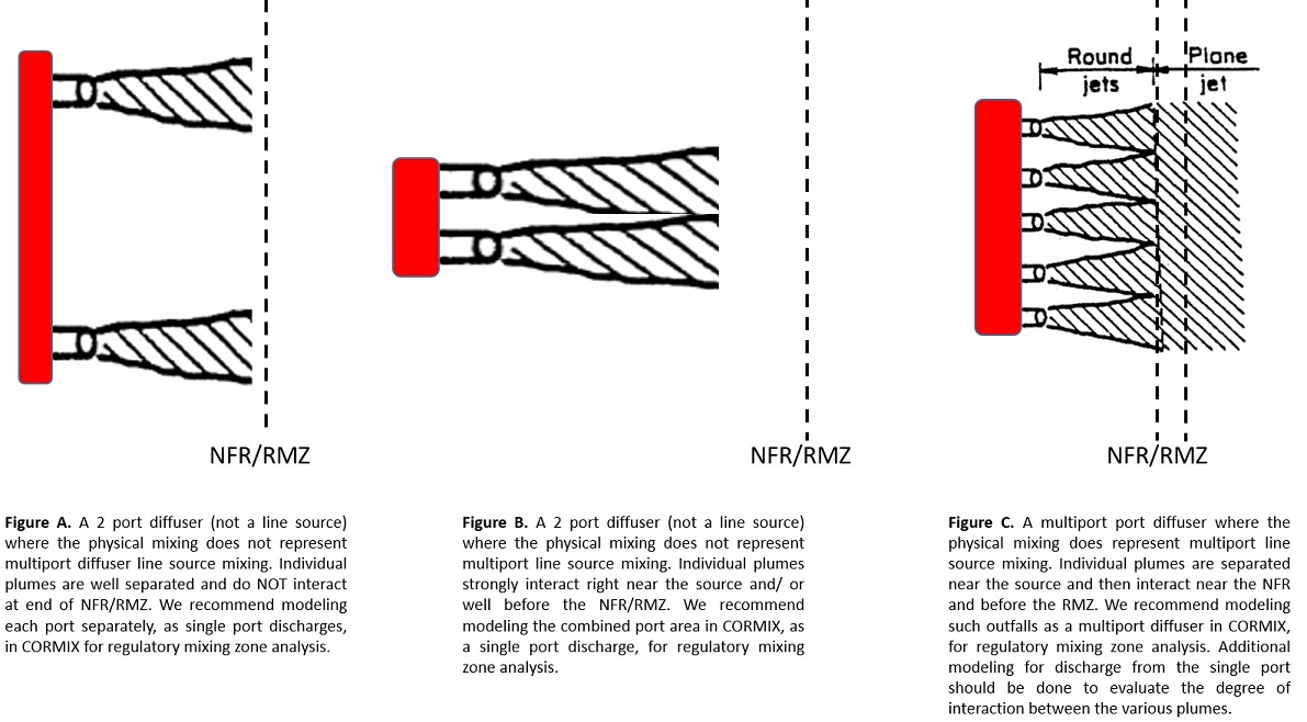
Q.30. Can CORMIX be applied to model accidental release (like a slug or pulse discharge) of effluent into ambient water bodies?
CORMIX is a steady-state, continuous point source discharge model, i.e. dQ/dt = 0 for discharge and ambient flowrates. Accidental discharges (like a slug release or pulse discharge) are not steady-state by definition. One can compare the accidental pulse duration (PD) of the effluent discharge to the travel time (TT) to the location where a dilution prediction is desired. If TT < PD, then a steady-state model like CORMIX may offer reasonable dilution estimates. However, if TT > PD, then dilution predictions may be underestimated.
Q.31. In sediment discharge cases modeled in CORMIX, why is there a difference in the predicted plume sediment concentrations and sediment mass fluxes remaining in the plume, along the plume trajectory?
The decrease in sediment concentration in CORMIX model prediction is due to an increase in physical dilution (due to mixing) AND due to
sediment particle settling (dependant on the particle density and fall velocities). However, the decrease in % of mass flux of sediment remaining in the plume is
ONLY due to particle settling. That is, even though the sediment plume is more diluted (decrease in suspended sediment concentration), it still has the sediment particles that have NOT yet settled out.
Q.32. Can CORMIX be used to model "timed" discharges (i.e. the effluent discharge occurs only for a few minutes or hours in a day)?
CORMIX is a steady-state, regulatory mixing zone model for continuous point source discharges.
It includes detailed near-field models with a simplified far-field modeling approach.
CORMIX can directly model the effluent discharge from a multiport diffuser
source (i.e., a single line source with multiple effluent discharge ports).
Q.34. What is the justification for the use of the "equivalent slot diffuser" concept in CORMIX to model certain multiport diffuser line source designs?
Depending on the multiport diffuser design being modeled, the CORMIX predicted flow classification, and mixing complexity, the CORMIX2
model can simulate the discharge from a multiport diffuser line source as multiple individual plumes before and after merging or as a two-dimensional plume from an
"equivalent slot diffuser".
Q.35. What is a "Control Volume" and why are there only two sets of plume trjectory prediction points (one set for inflow and the other for outflow) in certain CORMIX predictions?
In fluid mechanics, a control volume is a mathematical abstraction used when developing numerical models of complex physical processes.
Control volumes in CORMIX are used to represent plume boundary interactions with the surface, bottom, or a density stratified terminal layer.
Control volumes are also employed to model unstable circulation regions. Generally, length scales are used in
control volume techniques to simulate complex flows where more detailed methods are unavailable.
Q.36. Why are the predicted plume (half) widths, BH, greater than the schematized ambient cross-section width, BS, in the near-field, in certain CORMIX simulations?
CORMIX is a regulatory mixing zone model and assumes that there is enough lateral ambient mixing water
in the near-field for initial
dilution to occur (in general, most rivers and streams where regulatory mixing zones are applied are much wider than they are deeper).
Hence, within the near-field, the CORMIX model does not check for plume lateral boundary interaction.
It does check for discharge plume stability
and dynamic attachments due to vertical
boundaries (bottom, surface, pycnoclines, and stratified ambient density profiles) within the near-field.
Yes, CORMIX may be used to model the physical mixing of TSS in effluent discharges in ambient receiving waters.
The CORMIX model predictions of TSS assume that the TSS effluent concentrations get diluted by ambient entrainment
just like any other dissolved pollutant, when TSS concentration in the effluent is entered as excess above the ambient
background TSS concentration.
|
|||